Multiple Dependent Data Validation Drop-down Lists

Data Validation drop-down lists are a powerful Excel feature. Creating a list of items for the user to select from is not only an efficient way to input data into a cell but also ensures that the data going into the cell is the same every time, helping to keep the spreadsheet error-free and consistent. 

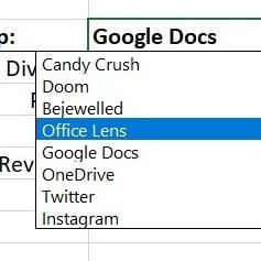
In the above example, I have created a single data validation drop-down list to make it simple for anyone to select an app and input it into the cell. 

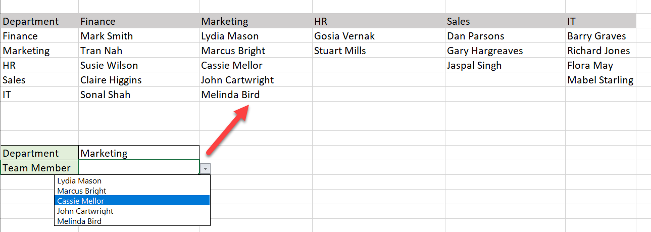
However, what if you want to have multiple dependent drop-down lists? In the example below, the ‘Team Member’ drop-down list is dependent on the selection made in the ‘Department’ drop-down list. If I were to select ‘Sales’, the list of team members would update to show the team members in that particular team. 
 

There are many ways to create dependent drop-down lists so let us look at a couple of them. 

Video Tutorial

Example 1: Creating a Dependent Drop-down List

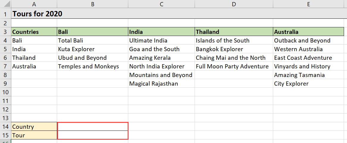
In this example, I am going to use the INDIRECT function to create two dynamic data validation drop-down lists. I am aiming to create a drop-down list in cell B14 that lists the countries and a drop-down list in cell B15 that lists the tours available in whichever country has been selected in cell B14. 
 

Creating Named Ranges

To make this easier, I am going to create a named range for ‘Countries’, ‘Bali’, ‘India’, ‘Thailand’, and ‘Australia’.  

1. Select the Countries, cells A3 to A7
2. Click the Formulas tab
3. From the Defined Names group, click Create from Selection
4. Select Top Row

NOTE: The selection you make here determines the name of the named range. 

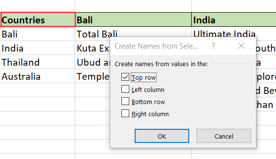
1. Click OK
2. Repeat steps 1 to 5 for 'Bali', 'India', 'Thailand', and 'Australia'
    

Creating Drop-down List 1

Let’s now set up the first drop-down list using Data Validation. 

1. Click in cell B14
2. Click the Data tab
3. From the Data Tools group, click Data Validation
4. Select List in the Allow drop-down
5. In the Source, enter =Countries
    

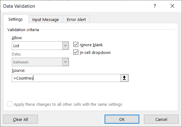
1. Click OK
2. A drop-down list will now appear in the Country field. 
    

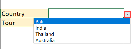
Now, we need to create a second list to display the Tours. This list will dynamically change depending on the Country selected. 

Creating Drop-down List 2

Let us now create the second drop-down list which is dependent on the selection made in the first. To do this we are going to use Excels INDIRECT function. 
 

1. Click in cell B15
2. Click the Data tab
3. From the Data Tools group, click Data Validation
4. Select List in the Allow drop-down
5. In the Source, type =INDIRECT($B$14)
    

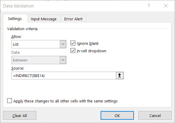
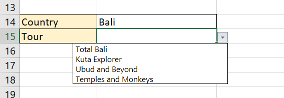
The INDIRECT formula references the country listed in cell B14 and matches it to the named range of the same name to produce the correct drop-down list. 
 

Example 2: Creating Expandable Dependent Drop-down Lists

The previous example is a great way of creating a drop-down list using named ranges, data validation, and the INDIRECT functions, however, it does have some drawbacks. Named ranges are fixed so if you update your data, add new data in, etc. then you would need to edit the named range to include the new data. This can be quite time-consuming and inefficient. 

In this example, I am going to show you how to create expandable dependent drop-down lists that will automatically update when new data is added. 

Format Data as a Table
 

1. Click within the data
2. Press CTRL+A to select all
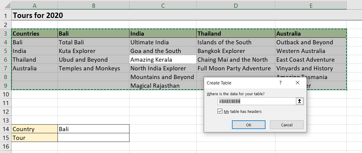
3. Press CTRl+T to create a table ensuring you have selected the checkbox ‘My table has headers’ selected
4. Click OK
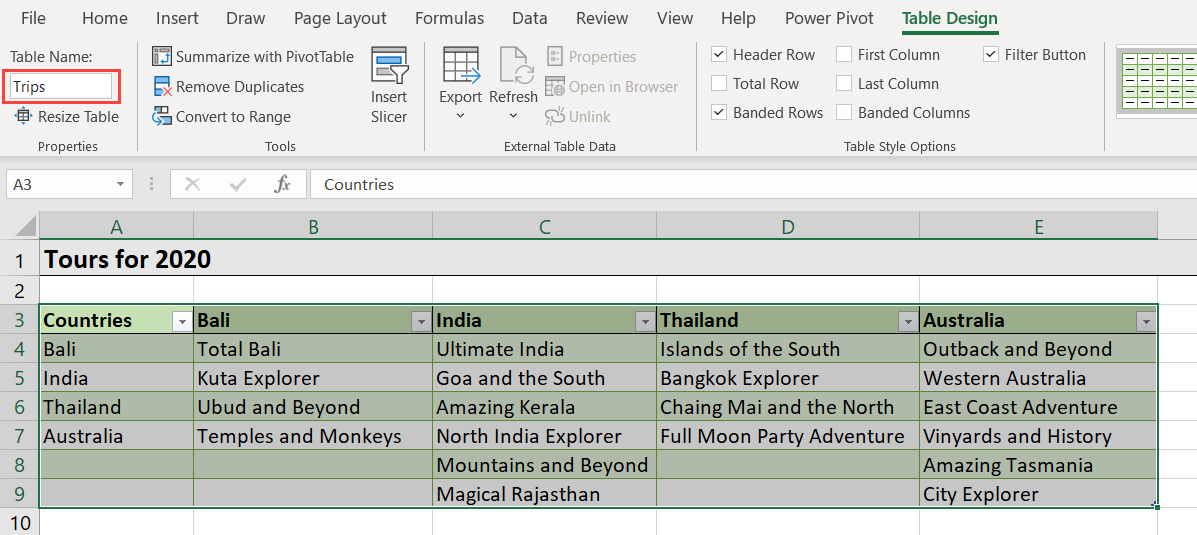
5. From the Table Design ribbon, in the Properties group, name the table and press Enter
    

Create a Named Range

Tables expand to accommodate new data BUT you cannot link directly to them from the Data Validation dialog box. So, we must also create a named range which we can link to. 

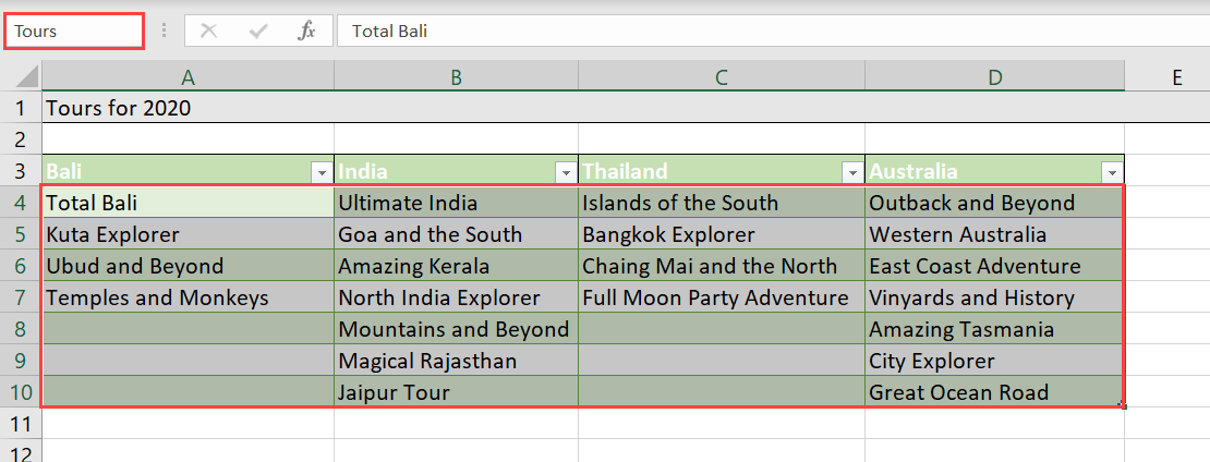
1. Select all the data excluding the heading row
2. In the Name box, give the range a name
    

Create the First Data Validation Drop-down List

First, we need to create a list that shows the countries. 

1. Click in cell B14
2. Click the Data tab
3. From the Data Tools group, click Data Validation
4. Select List from the Allow drop-down
5. In the source field, type = and select row 3
6. Click OK
    

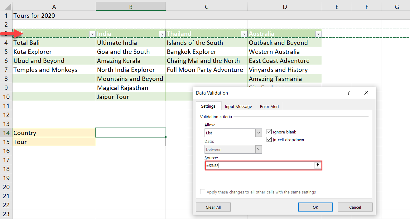
NOTE: Selecting the entire row ensures that any new countries added will be included in the drop-down list. 

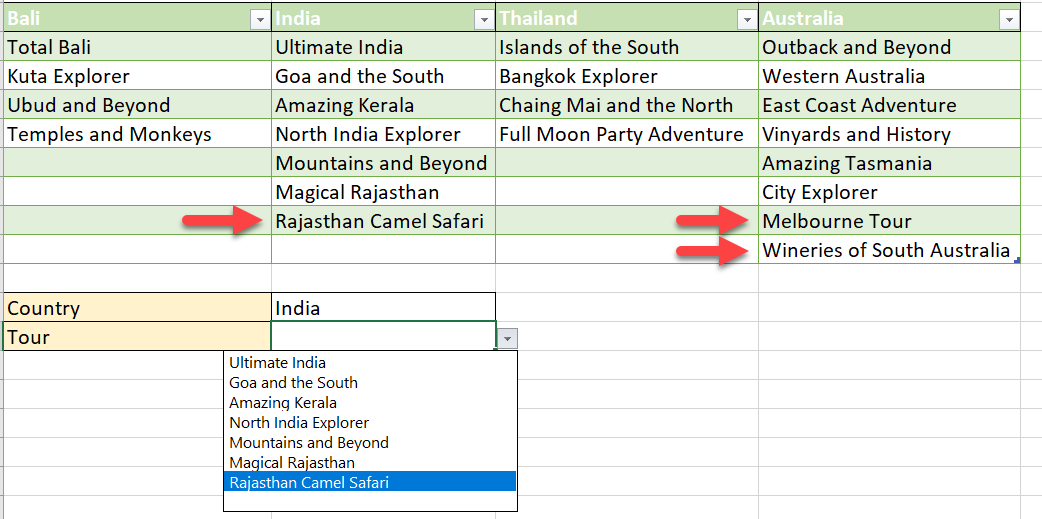
Create the Second Data Validation Drop-down List

Next, we are going to use the INDEX and MATCH functions along with Data Validation to create a list that expands when new items are added. You can practice the formula in a cell in the worksheet to ensure it works and then copies it into the Data Validation dialog box if you want to. 

1. Click in cell B15
2. Click the Data tab
3. From the Data Tools group, click Data Validation
4. Select List from the Allow drop-down
5. Type the INDEX/MATCH formula 

NOTE: Remember, you can press the F3 key to bring up a list of named ranges 

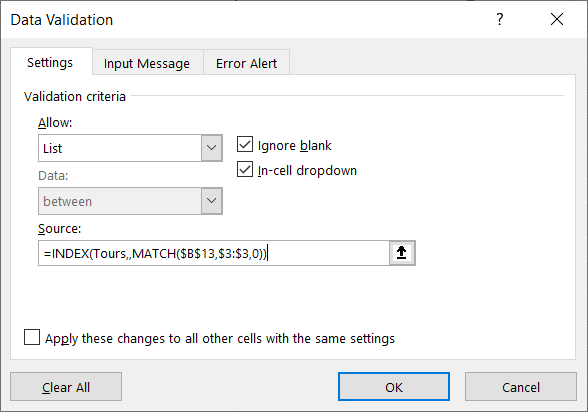
1. Click OK
2. When new data is added, it now appears in the drop-down menu. 
    

These are just a few examples of how to create multiple data validation drop-down lists. 

To learn more about important features in Excel, check out our courses on Michael Management.